Quick Lens Tutorial for Building FeedForward
Networks
Starting basics.
Lens, the Light Efficient Network Simulator, is a C program for running neural network simulations. The main user interface for the program is built in TclTk, a scripting language that is fairly easy to learn and makes it easy to manage certain kinds of graphical displays. The main command-line console in Lens takes TclTk commands in addition to specialized commands for building, training, testing and displaying networks. What Lens does is to execute a series of such commands in a particular order. The commands can either be typed directly into the command-line console window, or saved in a text file. If saved in a text file, you can tell Lens to “source” the text file, in which case the commands it contains will be executed in the order they appear in the file.
Lens comes with a comprehensive html-format manual included as part of the standard distribution. The manual provides copious detail which can sometimes be an impediment to getting your head around the simulator’s basic functionality, especially if you have had little or no computer programming experience. The purpose of this brief tutorial is to give you a sense of the basic steps for building your own feed-forward network, and some information about how each of the steps works. This tutorial omits many of the details and nuances that make Lens powerful; however it should provide enough information to help you navigate the Lens manual to find further detail.
For those who prefer to get all the detail from the beginning I recommend reading the manual pages in an order that is not intuitive given the layout of the main manual web page. Specifically:
Introduction
Tutorial network (under Example Networks)
Building and initializing networks (under Special Topics)
Group types (under Special Topics)
Example files (under File Formats and Usage)
Training standard networks (under Special Topics)
Weight files (under File Formats and Usage)
…by this time you should have enough basic information under your belt to make good use of the manual’s Command Reference, which lists all Lens-specific commands, provides a brief description of the functionality, as well as links to the detailed manual page for each command.
The rest of this mini-tutorial takes you through the various steps for building a feed-forward network.
Step 1: Build your network.
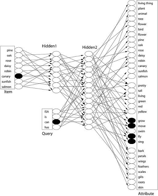
It’s a good idea to begin with a drawing of the network you want to build to use as a reference as you put the commands together. Let’s build a version of the Rumelhart semantic network that was exhaustively analysed by Rogers and McClelland(2004). A drawing of the network appears here.
The network has two input layers (Item and Query), two hidden layers, and one output layer (Properties), with connections as indicated in the figure. The network can be trained to answer different 4 different queries about each of the 8 items. Each item is represented by a single input unit in the Item layer, and each query is represented by a single unit in the Query layer. To ask the network what a canary can do, we activate the “canary” unit in the Item layer and the “can” unit in the Query layer. Activations feed forward from these inputs, ultimately activating some units in the Properties output layer. If the weights are set appropriately, the network will only activate those properties that represent what the canary can do (e.g. “fly,” “sing”, “move”).
There are only two parts of your work that you can save in Lens: the weight matrix for a network, and the set of examples you are working with. You cannot save your network. Instead, you build a network from scratch every time you run a Lens session. You can do this by typing the various build commands into the command-line console every time, but this will obviously get pretty tedious. Instead what you should do is write the series of commands to build your network in a text editor, and save the file. You can then tell Lens to read the file and execute the series of commands in the order they are typed in the file. To do this, you use the “source” command. For instance, if the commands to build your network were stored in a text file called stupid.net, you would run the list of commands by typing the following into the Lens command console:
source stupid.net
…as long as the text file is in the same directory where you invoked Lens, this will work. If the file is in another directory, you need to specify the full path to the file. In what follows, we will type the commands to build our network directly into the command console; at the end we will save them all in a text file and run them from there.
Building a feedforward network in Lens involves three basic commands:
addNet which creates and names the network object and sets many default parameters.
addGroup which will add layers of units to the network object and set default parameters for the groups added
connectGroups which will add weights between layers and set default parameters for the weights.
The addNet command takes arguments that will automatically add layers and connect them together, so you can actually create simple networks with a single command. We will build our network with the three commands above, and then look at how to use this shortcut.
Create the network
addNet
rumelhart
Use this to tell Lens you want to build a network named “rumelhart”. If you just type this into the console, a feedforward network with default parameters will be created. It will have a single layer with a single unit which is used to store bias weights in the rest of the network; it will not have any layers that you can use. For recurrent networks (ie networks that behave over time), there are additional arguments you need to supply that will control the network’s temporal behavior. But since we are concerned with feedforward networks, you can ignore these arguments. You must, however, specify a network name.
Type the above command directly into the Lens console. Various buttons on the main window of the graphical interface can now be clicked. Click on “New Object Viewer.” This window shows you the structure of the network object just created, and all of the data fields attached to the object---for instance, the number of groups (layers) it has (just 1), the number of input units (none), number of output units (none), etc. You can use this window to investigate all of the objects that exist in the current Lens session. For now, close the window.
You can have more than one network in existence in any Lens session. Only one network at a time can be the “active” network, ie the one that current commands will be directed towards. If there is only one network in existence, it is automatically the “active” network. You can use the useNet command with no arguments to list all currently existing networks. Use the same command to change the currently active network by providing the network name as an argument.
Just for fun, let’s make a second network:
addNet
stupidnet
When you add a new network, it automatically becomes the active network—you can tell because its name appears at the top of the main control window. Now list the networks:
useNet
…and switch back to rumelhart as the active network:
useNet
rumelhart
In fact, let’s get rid of the second network all together:
deleteNets
stupidnet
You can check to make sure it has been deleted (hint: useNet again).
Add layers to the network
addGroup
item 8 INPUT
addGroup
query 4 INPUT
addGroup
hidden1 8
addGroup
hidden2 16
addGroup
properties 32 OUTPUT SUM_SQUARED -BIASED
These commands add 5 layers to the currently active network. After each addGroup command comes the layer name (hey, they are named just like the layers in the Figure!), followed by the number of units in the layer. After the number of units can come a series of parameter options, in the form of words in UPPER CASE LETTERS. These determine just what kind of units are created in the group. Most obviously, INPUT means the layer is an input layer (it can take external inputs from the environment) and OUTPUT means the layer is an output layer (it can receive training targets from the environment). It is possible to have layers that are both input and output—just specify both parameters when you create the layer (e.g. addGroup stupidlayer 25 INPUT OUTPUT). This doesn’t make much sense in a feed-forward network so don’t do this now. In a recurrent network, where activation can flow in any direction, this property is useful.
There are many other parameters you can specify at this
level, described in the manual (look up addGroup in the command index). Where no parameters are
specified, default parameters are selected as also described in this part of
the manual. For instance, if neither INPUT nor OUTPUT is specified, the network
by default creates a hidden layer that cannot receive external inputs or targets.
Parameter specifications can be used to set the activation function (e.g.
specifying LINEAR will create a linear activation function for all units in the
group; specifying EXPONENTIAL creates an exponential activation function, etc.
By default the activation function is sigmoidal). You
can change how inputs are calculated—the default is dot-product (ie the product of sending activation and incoming weight,
summed across all sending units) and you will probably stick with this for most
networks but you can play around with the other options described in the
manual. You can specify how external inputs are applied to input units—are the
input units directly set to value specified by the environment (HARD_CLAMP, the
default), or is the external input just added in to the net input of the unit (
Two parameters important for the output layer of the current model are specified in the commands above. First, Lens by default uses a measure of error on the output units called “cross-entropy.” This measure seriously penalizes output units for being on the wrong side of 0.5 (ie, if they are near 0 when they should be 1, the error approaches infinity). We are going to use the squared-error function familiar from our derivation of the delta rule. To do this in Lens, we specify the SUM_SQUARED parameter when we create the output layer. All units in this layer will now compute sum-squared error as their measure of error instead of cross-entropy.
Second, all units except input units by default get a “bias weight”—that is, a weight from a single unit that is always one, which can be trained. The bias allows the model to set unit activations to their base activation—their average activation across all training examples—even in the absence of any input. We don’t want the model strongly activating frequently-occurring output properties in the absence of any input, so we want to tell the model not to create bias weights for the output units. This is accomplished by specifying –BIASED. By default, the output units have the BIASED parameter specified—the minus sign in front of the word BIASED tells it to refrain from this default behavior.
You can look at the groups you have created using the New Object Viewer. Click on this button again and look at the numGroups field: it now says 6, indicating that you have created 5 new layers in addition to the original bias layer that is automatically generated. Similarly, numOutputs indicates that there are 32 output units; numInputs indicates that there are 12 inputs (8 items and 4 query inputs). Now click on the Group button. You can select which group you want to examine—let’s pick “item.” The display changes to show you the item group (ie the first input layer) and all of the parameters associated with this object. For instance the “net” field shows that this group belongs to the rumelhart network; numUnits shows that there are 8 units in the group, etc. You can further navigate down the object chain by clicking on “Unit” and selecting one of the 8 units in this group. The resulting display shows you all the parameters associated with this individual unit. Finally, you can go back up the hierarchy using the funny-looking triangle buttons at the top of the viewer window. In general you can inspect all of the parameters for all of the currently existing objects in this viewer. Obviously, there are a lot of parameters and not all of them will be relevant to what you are currently doing—but it is reassuring to know the information is all there. For now, go ahead and close the window again.
Connect layers together
connectGroups
item hidden1 hidden2 properties
connectGroups
query hidden2
To add links (ie weighted connections) between units in different layers, type in the commands above. When no parameters are specified for the connectGroups command, Lens will connect every unit in layers toward the left of the list to every unit in layers toward the right. In the first command above, all item units will send connections to all hidden1 units; all hidden1 units will send connections to all hidden2 units; all hidden2 units will send connections to all properties units. For the Rumelhart semantic network, you need a second connectGroups command to connect the query layer to the hidden2 layer, because there is no way of indicating this connection in the first command that will lead to the correct pattern of connectivity.
There are several parameters you can specify that will
influence exactly what patterns of connection will be created. Just as
previously, these parameters are set by typing them in in
UPPER CASE LETTERS on the same line as the connectGroups
command. All links created by that particular command will conform to the
parameter specifications that follow. The default choice is full connection:
all units in the sending layer are connected to all units in the receiving
layer. Other specifications will create other patterns of connectivity, and
these are clearly documented in the manual page for the connectGroups
command. Some examples include RANDOM (will generate connections between pairs
of sending and receiving units with probability S) and
Viewers
You can see your network and the links created using the Unit Viewer and the Link Viewer in the graphical interface. To plot the network you have created, try:
autoPlot
16
autoPlot will created a display in which layers are shown as sets of squares, and empty spaces appear between layers. To see it, click on the UnitViewer button in the main interface window. Layers will be plotted from the bottom up (ie layer 1 at the bottom, layer 2 above it, etc.). The number following the autoplot command indicates how many columns you want to appear in the plot. Contrast the display produced by the above command to the one produced by: autoPlot 8. If you don’t like the plots created by autoPlot, you can gain more fine-grained control over the display using a series of plotting commands described in the Unit Plotting Commands part of the Command Reference in the manual.
To view the links in the network, just click the LinkViewer button in the graphical interface. A matrix appears indicating all pairs of units, with sending units listed down the left from the last unit in the net at the top to the first unit at the bottom, and receiving units across the top from the last unit at the left to the first unit at the far right. Wherever a link exists between units, a colored square appears showing the value of the weight. To see the exact value, move your cursor over the link; the actual value appears in the corresponding field at the top of the link viewer window. You can use the link viewer to verify that the network is connected properly: for instance, that the item layer sends connections to hidden1; that query connects to hidden2; and so on.
Shortcuts
Okay, you have built your network. Do you have to go through this whole thing every time you start up Lens? Of course not. You can save the series of commands in a text file, and then tell Lens to “source” the text file the next time you want to rebuild the network. Just type the series of commands above, in order, into any text editor and save the file in the directory where you want this work to be stored. For your convenience, I have done this here. You might rename it rumelhart.net. Quit Lens, navigate to the folder where the text file is stored, and start Lens again. Now type this into the console:
source rumelhart.net
Lens runs through all the commands stored in the text file as though you have typed them into the console. You have rebuilt and reconnected the Rumelhart network!
Finally, the addNet command takes a set of arguments that allow you to skip the addGroup and connectGroups commands for feedforward networks with simple connectivity. After the network name, you simply specify a series of numbers and parameters. For each number supplied, the command will add a group with the corresponding number of units. The first such group will be of INPUT type, the last will be of OUTPUT type, and intermediating groups will be hidden layers unless specified otherwise. Parameters specified after each will be applied to the corresponding group; and links will be created amongst groups connecting those on the left to those on the right. For instance:
addNet stupidnet
…will create a feed-forward network with 10 input units, a hidden layer with 20 sigmoid units (the default), a second hidden layer with 20 linear units (specified by LINEAR above), and 5 output units that use sum-squared-error.
Step 2: Creating the environment
Congratulations, you have a network. But wait, you are not done. Your network is no good unless you have a set of patterns for it to process. To create such patterns, you need to create an example file—a text file that lists the inputs and targets for every pattern. You do not generally create this file in Lens (though it is possible to do so); you create it using your favorite text editor, save it, and load the examples later in Lens.
Example files for recurrent networks, which may consist of complex sequences of events, can get complicated. For feedforward nets they are relatively straightforward since each event consists of a single input pattern and a single output (target) pattern.
The example file consists of 2 parts: an optional header, which sets default values for the patterns, and the examples themselves. There are 4 commands you might want to include in the example file header:
defI 0.0 Sets the default value for input units.
defT 0.0 Sets the default value for targets.
actI 1.0 Sets the default value for an active input unit.
actT 1.0 Sets the default value for a target unit that should be activated.
These set the default values for the patterns, so you don’t have to specify them directly in the individual examples. There are other pieces of information you can put in the header which you can read about in the Example Files section of the manual. For now, type the four lines above into the text editor, followed by a semicolon. The semicolon tells Lens that the header is finished; if you omit the header all together, you can leave out the semicolon as well.
After the header comes the list of examples specifying the inputs and targets for each pattern, as well as (optionally) a name and a frequency for each pattern. There are 2 different ways to specify the individual examples.
Dense coding
For dense coding you type in the actual values of the inputs and targets for all input and output units that take on a value other than the defaults set in the header. The syntax looks like this:
name: rose_is freq: 2 I:
0 0 1 0 0 0 0 0 0 1 0 0 T: 1 0 1;
The optional name: specification allows you to name the pattern; the optional freq: specification indicates that the pattern should appear twice in a sweep through the full training corpus, although this will be ignored unless the training set is sampled probabilistically (see below). The I: indicates that you are going to specify the pattern of activity across input units, beginning with the first; and the T: indicates that you are about to specify the pattern of targets across output units, beginning with the first. Note that, even though there are 2 input layers in the network, this is not reflected in the example file. Instead the input layers are effectively “strung together” in the order they are created and treated as one long vector for the example file. In the current network the first 8 values following I: will be applied to the 8 units in the first input layer (item) and the remaining 4 will be applied to the next input layer (query). The same is true of target patterns for networks with more than one output layer.
Also note that, although there are 32 output units in our network, we only specified 4 target values. In a given event, any input or output units not assigned explicit inputs or targets will receive the input and target values specified by the defaults in the header. In this case, unspecified inputs and targets will both receive the value 0.0. Since all 12 inputs have specified values, the only unspecified visible units are the 28 remaining units in the output layer, which will all receive a value of 0.0. If for a given event you want to use default values other than those indicated in the header, you can give a pattern-specific default value by putting it in curly braces at the beginning of the pattern:
name: rose_is I: {.5} 0
0 1 0 0 0
0 0 0
1 T: {.3} 1 0 ;
…here unspecified input units will take on the value 0.5 and unspecified targets will take on the value 0.3.
The event description ends with a semicolon. Another event can be created by adding another similar line to the event file, ending in a semicolon; and each such line will create another event in the set. If you want to have different input and/or target values for different units in the same pattern, you must use this dense coding format for the patterns.
Sparse coding
In the sparse coding format, you do not specify the actual values of the inputs and targets. Instead, all inputs and targets will have default values specified either in the header or at the beginning of the example, and each example line simply tells Lens which input units and targets should be active in a given pattern.
name: rose_is i: 2 9 t: 0 3;
The above command will produce the same pattern as the dense coding example shown above. Basically it is saying: create a pattern called “rose_is”, in which input units 2 and 9 are turned on and all other inputs units are turned off; and output units 0 and 3 have active targets and all other output units have deactivated targets. NOTE that units are numbered beginning with 0 in the example file—so the first ten units in an input layer are numbered 0-9 in the example file. The values for an active input and target are specified in the header settings for actI and actT, respectively; the values for deactivated inputs and targets are specified in header settings for defI and defT, respectively. The default active values can also be specified for each pattern separately using curly braces just as previously:
name: rose_is I: {.75}
2 9 T: {.95} 0 3;
…this will set inputs 2 and 9 to the value .75, and targets 0 and 3 to .95. Note that in this case, you must use UPPER CASE I: and T:. Only if there are no values in curly braces should you use the lower case format i: and t:—don’t ask me why.
Here is a sparse specification of a
set of training patterns for the Rumelhart network. These
are not the actual patterns used in
the
loadExamples
rumelhart.ex
If all went well, you should be able to click on the UnitViewer button in the main graphical interface to bring up the graphical display of the network. All of the examples should now appear down the left side of the display. To see how the network processes an example, just click on it. The network display shows the activations of all units in response to the input using color shades ranging from blue to black to red. The target values for the output units are indicated by the colour of the boundary surrounding the square that represents each output unit.
It is worth reading the manual page for the loadExamples command, because this command takes arguments that determine how the patterns in the example set will be ordered and sampled during training. By default, patterns are presented to the network in the order they are listed in the example file. You can have them presented in randomly permuted order by loading the set as follows:
loadExamples
rumelhart.ex PERMUTED
Other options include RANDOMIZED (purely random selection) and PROBABILISTIC (each pattern appears in the set with a likelihood specified by the freq: fields in the example file). For training, you typically want the sampling to be PERMUTED if there are no frequency differences among the items in the set; or PROBABILISTIC if frequencies are specified.
You can have multiple example sets loaded into Lens at any given time. The first set loaded will automatically be classified as the “training” set (the set used when the training commands are invoked); the second set loaded will automatically be used as the testing set (the set used when testing commands are invoked). You can load the same set twice with different parameters for training and testing. For instance:
loadExamples
rumelhart.ex
loadExamples
rumelhart.ex
…will load the example set with a permuted samping into the training set, and will load the same examples with the default non-permuted sampling into the test set.
At this point you have your network built and connected, and your training and testing patterns loaded in, so you are pretty much ready to start training and testing the network.